These are some of my notes on the distributed memory model and MPI collectives that are discussed in Georgia Tech’s CSE6220 High Performance Computing course. Main goal here is to lay down a brief synopsis on these topics to help me prepare for the final exam, so if you’ve stumbled on these notes some how and want to learn more, I recommend the following resources:
Distributed Memory Model
The Distributed Memory model is an abstraction for dealing with problems that are too large to fit on a single machine. Essentially it just describes a networked cluster of individual computers each with their own private memory that the other machines cannot access. This means that these networked computers must communicate with each other to share messages and data. This is called “message passing” (hence the whole Message Passing Interface!).
Basic Rules of the Model
In this course, we assume the following rules about the distributed memory model hold.
- All nodes in the network are fully connected
- All links in the network are bidirectional
- Each node can at most send + receive one message at a time (it can send/receive simulatenously because of the bidirectional links)
- Cost to send/receive
nwords (in a message) – Tmsg(n) = α + βn - K-way congestion reduces available bandwidth – Tmsg(n) = α + βnK
Alpha-Beta Model
The Alpha-Beta Model helps us account for the cost of communication when analyzing the time of an algorithm. Let’s break down the following:
Tmsg(n) = α + βn
As mentioned earlier, this equation represents the cost in Time it takes to send/receive a message of n words.
- Alpha (α) - represents the network latency cost of the message (time/message). It is a constant factor for each message sent.
- Beta (β) - represents the inverse bandwidth cost to send each word of the message (time/word). It grows linearly with the size of the message.
- Tau (τ) - is not present in the equation above, but it represents the cost of the computation performed by the algorith.
In practice, the relative costs of these factors are as follows:
τ < β < α
So the cost of local computation is cheaper than the cost of bandwidth which is cheaper than the cost of fixed network latency. This means that an algorithm that avoids unnecessary communication and favors fewer large network requests over many smaller ones will often be more performant.
MPI Collectives
As mentioned earlier, the MPI Tutorial is a better place to learn more about these and how to actually use them in practice. The notes below will mostly consist of brief explanations, use cases, and other tidbits. Note: P indicates the number of procesessors communicating with each other and rank indicates an individual processor’s id amongst the others.
The lectures also introduce the concept of a collective having duals. A dual in this context is a related collective that behaves similarly, but in reverse. For example, the All-to-One reduce’s dual would be the One-to-All Broadcast. When possible I will note a collective’s dual along with it.
Lower Bound on Communication for MPI Collectives
T(n) = Ω(⍺*log(P) + βn)
We can use tree-based or butterfly style communication to cut down on the amount of discrete send operations between nodes which can help us reduce the cost of alpha from ⍺*P to ⍺*log(P).
All-to-One Reduce
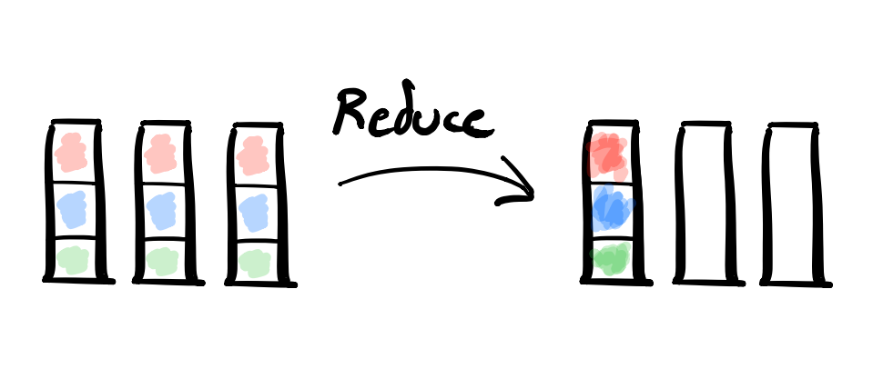
- MPI Collective: MPI_Reduce
- Description: An All-to-One Reduce takes a reducing operation (e.g.
sum) and uses it to reduce data from all processors down to a single “root” processor. - Example Usecase: Consider a dataset that is too large to fit in memory on a single machine – like we’re counting words in a large text corpus. You might distribute it across multiple processors and then use an All-to-One Reduce to reduce the counts down and send to the leader node.
- Dual: Broadcast
One-to-All Broadcast

- MPI Collective: MPI_Bcast
- Description: A (One-to-All) Broadcast takes data that is on one root node and sends copies of it to every other node.
- Example Usecase: Consider a single machine that has performed an exceptionally computationally expensive task (τ > α + βn). In this case, rather than make P processors also perform the computation we might use a Broadcast to distribute the computed result.
- Dual: All-to-One Reduce
Scatter

- MPI Collective: MPI_Scatter
- Description: A Scatter distributes chunks of data from the root node to all of the other processors.
- Example Usecase: Consider the root node at rank 0 might have an Integer array of length P consisting of distinct counts it needs to send to every other processor. E.g.
[5, 3, 4, 9]. It could use a Scatter to send5to itself,3to the rank 1 processor,4to rank 2, and so on. - Dual: Gather
Gather

- MPI Collective: MPI_Gather
- Description: A Gather consolidates individual chunks of data from each processor on to the root node.
- Example Usecase: Consider each processor might have acquired a segment of data and performed some computation on it. This data makes up just one piece of a greater whole however. A Gather could be used to reconsolidate these segments onto a single node for further use.
- Dual: Scatter
All-Gather
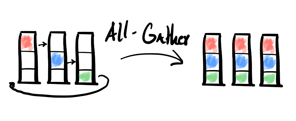
- MPI Collective: MPI_Allgather
- Description: An All-Gather is like a Gather followed by a Broadcast. It consolidates segments of data onto every processor.
- Example Usecase: Similar use cases to the Gather except every processor would find value in having the complete set of data, not just the root. A Broadcast could be implemented by a Scatter followed by an All-Gather.
- Dual: Reduce-Scatter
Reduce-Scatter
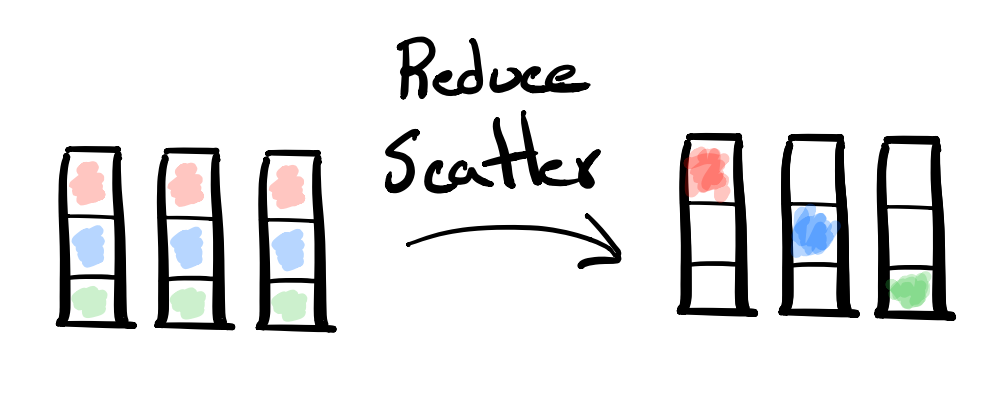
- MPI Collective: MPI_Reduce_scatter
- Description: A Reduce-Scatter is essentially a Reduce followed by a Scatter. So it applies some reduction operation across the data and then splits it up into segments to distribute to each processor.
- Example Usecase: If you find yourself needing to do a Reduce and distributing pieces of the output across to the processors, a Reduce-Scatter might be useful.
- Dual: All-Gather
All-To-All
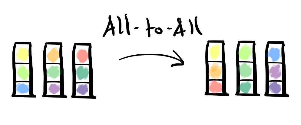
- MPI Collective: MPI_Alltoall; MPI_Alltoallv
- Description: All-To-All is a collective that allows each processor to send a different, specific piece of information to every other processor.
-
Example Usecase: In certain algorithms that use bucketing (e.g. bucketsort) you might have data distributed across every processor and need to consolidate specific pieces of data on specific processors. For example, say you have numbers ranging from 0-30. For your bucketsort you want the following buckets:
- Processor 0: n < 10
- Processor 1: 10 <= n < 20
- Processor 2: 20 <= n <= 30
Currently the processors contain:
- Processor 0:
[5, 16, 15, 7, 19, 18, 28, 4, 12, 13] - Processor 1:
[30, 1, 17, 24, 23, 21, 2, 26, 10, 14] - Processor 2:
[20, 8, 22, 6, 9, 11, 0, 27, 25, 3, 29]
You could sort each subarray locally on each processor such that it looks like this:
- Processor 0:
[4, 5, 7, 12, 13, 15, 16, 18, 19, 28] - Processor 1:
[1, 2, 10, 14, 17, 21, 23, 24, 26, 30] - Processor 2:
[0, 3, 6, 8, 9, 11, 20, 22, 25, 27, 29]
Then use an All-To-All (typically Alltoallv when the initial distribution isn’t uniform) to send the data to the correct buckets.
- Processor 0:
[0, 1, 2, 3, 4, 5, 6, 7, 8, 9] - Processor 1:
[10, 11, 12, 13, 14, 15, 16, 17, 18, 19] - Processor 2:
[20, 21, 22, 23, 24, 25, 26, 27, 28, 29, 30]